An fundamental but so-important point of view: Correlation is not causation
Main learning materials and reference:
[1] Pearl, Judea. Causality. Cambridge university press, 2009.
[2] Pearl, Judea, and Dana Mackenzie. The book of why: the new science of cause and effect. Basic books, 2018.
[3] Introduction to Causal Inference by Brady Neal,.
Correlation, or so-called associational relationship, absolutely should never imply the causation [1], while it is quite common for even some professional statistician to make this mistake. In fact, the debate between correlation and causation has persisted decades: A part of classical statistician, such as Francis Galton and Karl Pearson, insisted that causation is an “anti-scientific” subject [2]. As a result, related exploration was stalled for many years, and some exciting and gratifying advancements are observed still very recent years.
An intuitive (and ridiculous) example [2] to see the difference between correlation and causation is given by the plot below (Fig. 1):

(Source: https://www.tylervigen.com/spurious-correlations)
Obviously, the total revenue generated by arcades should not have any causal relationship with the number of awarded computer sciencec doctorates in US. However, the two figures strongly correlate in some coincidental way over the 10-year period. The problem without the causation’s support here is that the coincidence may fail in a very short future, which means it will be risky to use the revenue to infer the number of awarded doctorates empirically.
With the intuition of the difference between correlation and causation, we may further consider an interesting scenario [3] with the support of causal graph and some methmatical tools to distinguish thier differences. For instance, if we are curious about whether sleeping with shoes on will lead to the headache, and if so, how much the effect should be.
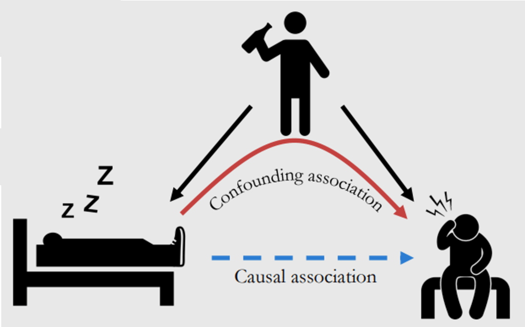
(Source: https://www.bradyneal.com/causal-inference-course)
Let’s start from the perspective of classical statistics that considers this problem in correlation view. The quantity that we would like to know according to the question should be ![E[Ache|Shoe = 1] - E[Ache|Shoe = 0]](https://s0.wp.com/latex.php?latex=E%5BAche%7CShoe+%3D+1%5D+-+E%5BAche%7CShoe+%3D+0%5D&bg=ffffff&fg=111111&s=0&c=20201002)

(Source: https://www.bradyneal.com/causal-inference-course)
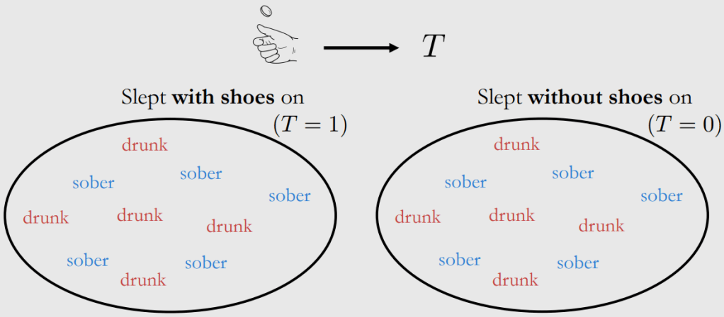
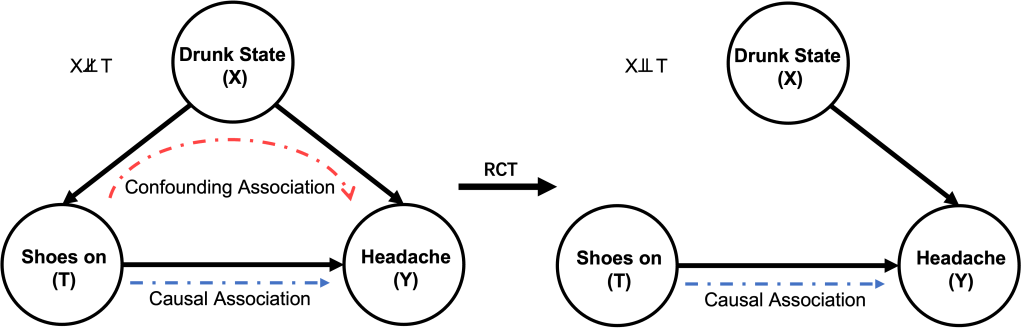
It may be feasible to conduct a Randomised Control Trail (RCT) here to remove the confounder of drunk state by, for example, rolling a dice or tossing a coin to randomly determine if a subject should wear his/her shoes on when sleeping whether they are drunk or not. In this way, the drunk state can be fairly distributed in both group (showing in Fig. 4), and thus this confounder will be removed (or saying blocked) in the causal graph above. In other words, treatment and control groups are the same in all aspects except treatment [3].
(Source: https://www.bradyneal.com/causal-inference-course)
Unfortunatly, in most of other scenarios, RCT is very difficult or just not possible to be conducted due to the fact that we may not be able to change what happened or the ethical limitations do not allow us to. For instance, it is immoral to enforce the subjects to smoke when we are investigating causal effect of smoking that leads to lung cancer (note that there might be other confunders that may cause the cancer, for example, unhealthy lifestyle and exccessive intake of porteins, to name but a few). Another example might be that the borad council once made a business decision, we can only observe the output of that decision, but cannot go back to the past and see what will happen if that decision was not made. This, in fact, is a common question that we always ask: what will happen if I did/did not do something, which is so-called conterfactual problem.
We, or more precisely — our brains, are able to deal with this kind of problem in a causal way. However, analysis purely based on correlation should not. That is why we have to introduce some adjustments to save the classical correlation-based statistics from a biased perspective to an unbiased causal perspective. Before we move to the next post which introduces some of the mathmetical tools to deal with challenge, an must-have term which needs to introducing here is the do-operator (
![\begin{aligned} ATE &= E[Ache|do(Shoe = 1)] - E[Ache|do(Shoe = 0)] \\& \neq E[Ache|Shoe = 1] - E[Ache|Shoe = 0] \end{aligned}](https://s0.wp.com/latex.php?latex=%5Cbegin%7Baligned%7D+ATE+%26%3D+E%5BAche%7Cdo%28Shoe+%3D+1%29%5D+-+E%5BAche%7Cdo%28Shoe+%3D+0%29%5D++%5C%5C%26+%5Cneq+E%5BAche%7CShoe+%3D+1%5D+-+E%5BAche%7CShoe+%3D+0%5D+%5Cend%7Baligned%7D+&bg=ffffff&fg=111111&s=0&c=20201002)
As an graphical representation, Fig. 5 below compares the difference between intervention and conditioning on the whole population. We use 
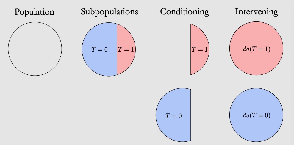
(Source: https://www.bradyneal.com/causal-inference-course)
Now, after knowing the differencec between conditioning and intervening, let’s take a step back to the RCT to understand why it can block the confounding effects. In the aforementioned example, if a subject will wear shoes on when sleeping (


If


And thus:

Fig. 6 below shows how the RCT changes the causal graph blocking all the confounding assocational paths (only one path in this example). In this simple causal graph, once the causal path between 

As discussed before, although RCT may not be valid all the time, causation indentification techniques and do-calculus can fill this hole. In particular, for some specific scenarios under certain assumptions, we may consider to use Back-door Adjustment and Front-door Adjustment to identify the causal relationships, which is easier to implement. In the next blog of Learning Record: Causal Inference, we may discuss these magical methods that help us travel from the correlation to the world of causation.
In conclusion, this blog seeks to clarify a key point of view that may change our ways of thinking: CORRELATION IS NOT CAUSATION, EXCEPT WHEN IT IS!. Bearing with this in mind, we will be able to interpret nowadays dazzling data from a totally different but more comprehensive perspective.
